Intro to TensorFlow in R - Edgar's Data Lab

TensorFlow is usually associated with neural networks and advanced Machine Learning. But just like R, it can also be used to create less complex models that can serve as a great introduction for new users, like me.

Training wheels

TensorFlow is a very powerful and flexible architecture. It provides the building blocks to create and fit basically any machine learning algorithm. But even a simple linear regression model has to be built “from scratch” using layers and estimators in TensorFlow.

TensorFlow has a high-level API that provides “canned models” which, in my opinion, lowers the barrier to entry into experimenting with TensorFlow. And of course, R users are now able to access this API via the tfestimators package.

Setup

TensorFlow and the R package are needed to use tfestimators in your computer or laptop:

Install tfestimators as follows:

devtools::install_github("rstudio/tfestimators")

tfestimators comes with a handy function that installs TensorFlow for you:
```
install_tensorflow(version = "1.3.0")
```

The model

The tfestimators package is the only one that will be loaded into R at this time.

library(tfestimators)

The plan

Define the feature columns (predictors)
Choose the model
Define the model inputs (response ~ feature columns)
Split the data into training and test
Train the model
Evaluate the model
Run predictions with the model

In R, most of these steps are usually covered in a single modeling function. And without the Estimators high-level API, these would be even more steps. The overall goal of this exercise is to introduce the workflow, and mindset needed to create Machine Learning applications using TensorFlow.

Refer to the full code if you wish to copy and paste it in your computer to follow along or test.

1. Define the feature columns (predictors)

Think of feature columns as the predictors or terms of a regular model. In this step, the type, values and other properties of the variable is defined. There are ten functions in tfestimators that can be used to prepare the definitions:

column_bucketized
column_categorical_weighted
column_categorical_with_hash_bucket
column_categorical_with_identity
column_categorical_with_vocabulary_file
column_categorical_with_vocabulary_list
column_crossed
column_embedding
column_indicator
column_numeric

Data from the familiar titanic package is going to be used for this example. Notice that the package, or the data, are not being loaded or called at this time. The reason is to highlight that the columns definition is not evaluated by R or TensorFlow in this step.

The Sex and Embarked variables will be defined as categorical, and their possible values are set by passing a list to the vocabulary_list argument. The Pclass variable is passed as a numeric feature, so there no further definition.

cols <- feature_columns(
  column_categorical_with_vocabulary_list("Sex", vocabulary_list = list("male", "female")),
  column_categorical_with_vocabulary_list("Embarked", vocabulary_list = list("S", "C", "Q", "")),
  column_numeric("Pclass")
)

2. Choose the model

There are five canned models, or estimators, to choose from:

linear_regressor
linear_classifier
dnn_regressor dnn_classifier
dnn_linear_combined_regressor
dnn_linear_combined_classifier

Calling the linear_classifier() estimator function starts the constructing the model. In this step, the only thing passed to the model are the feature columns variable, cols

model <- linear_classifier(feature_columns = cols)

3. Define the model inputs (response ~ feature columns)

The response and features columns are named as arguments in the input_fn() function. Notice that the variables named in features are the same defined in the cols variable.

titanic_input_fn <- function(data) {
  input_fn(data, 
           features = c("Sex",
                        "Pclass",
                        "Embarked"), 
           response = "Survived")
}

4. Split the data into training and test

In this step, the titanic_train data set is split into a train and a test data frames.

library(tidyverse)
library(titanic)

titanic_set <- titanic_train %>%
  filter(!is.na(Age))

glimpse(titanic_set)

## Observations: 714
## Variables: 12
## $ PassengerId <int> 1, 2, 3, 4, 5, 7, 8, 9, 10, 11, 12, 13, 14, 15, 16...
## $ Survived    <int> 0, 1, 1, 1, 0, 0, 0, 1, 1, 1, 1, 0, 0, 0, 1, 0, 0,...
## $ Pclass      <int> 3, 1, 3, 1, 3, 1, 3, 3, 2, 3, 1, 3, 3, 3, 2, 3, 3,...
## $ Name        <chr> "Braund, Mr. Owen Harris", "Cumings, Mrs. John Bra...
## $ Sex         <chr> "male", "female", "female", "female", "male", "mal...
## $ Age         <dbl> 22, 38, 26, 35, 35, 54, 2, 27, 14, 4, 58, 20, 39, ...
## $ SibSp       <int> 1, 1, 0, 1, 0, 0, 3, 0, 1, 1, 0, 0, 1, 0, 0, 4, 1,...
## $ Parch       <int> 0, 0, 0, 0, 0, 0, 1, 2, 0, 1, 0, 0, 5, 0, 0, 1, 0,...
## $ Ticket      <chr> "A/5 21171", "PC 17599", "STON/O2. 3101282", "1138...
## $ Fare        <dbl> 7.2500, 71.2833, 7.9250, 53.1000, 8.0500, 51.8625,...
## $ Cabin       <chr> "", "C85", "", "C123", "", "E46", "", "", "", "G6"...
## $ Embarked    <chr> "S", "C", "S", "S", "S", "S", "S", "S", "C", "S", ...

indices <- sample(1:nrow(titanic_set), size = 0.80 * nrow(titanic_set))
train <- titanic_set[indices, ]
test  <- titanic_set[-indices, ]

5. Train the model

This is where all of the previous steps come together. The train() function is used to fit the model.

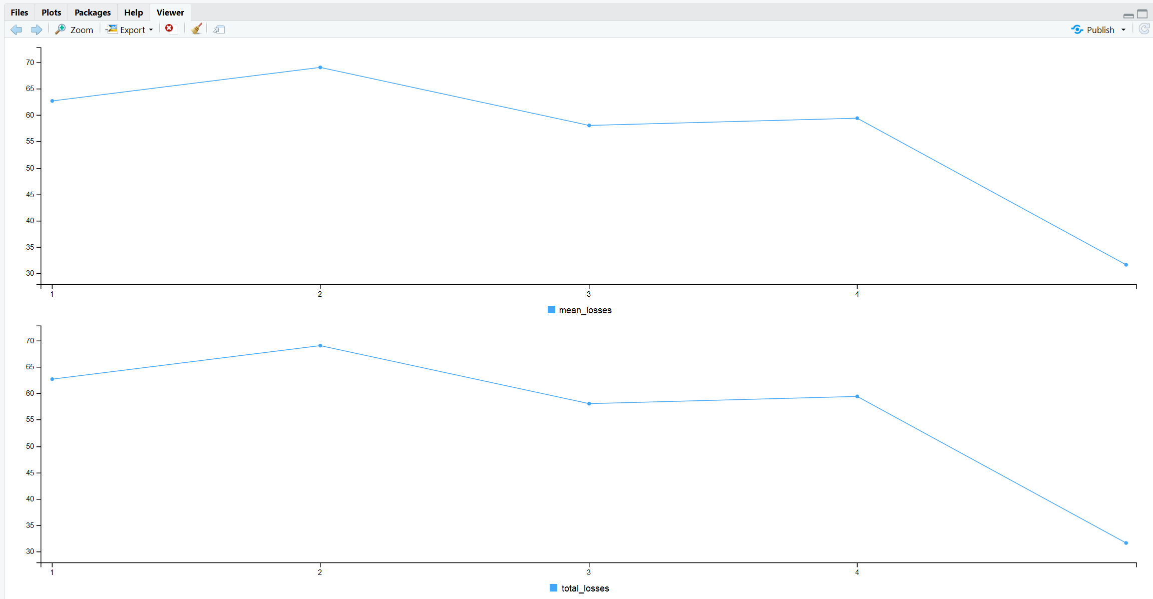
train(model, titanic_input_fn(train))

Notice that the the results are not being passed to a variable. The train() function does the following:

Fits the model. This is a typical message returned to the console:

[-] Training -- loss: 26.80, step: 5

Returns two plots to the R viewer.

Saves the results to the file system. The model’s path can be found in this attribute: model$estimator$model_dir

list.files(model$estimator$model_dir)

## [1] "checkpoint"                                    
## [2] "events.out.tfevents.1508693806.DESKTOP-10DBTVP"
## [3] "graph.pbtxt"                                   
## [4] "model.ckpt-1.data-00000-of-00001"              
## [5] "model.ckpt-1.index"                            
## [6] "model.ckpt-1.meta"                             
## [7] "model.ckpt-5.data-00000-of-00001"              
## [8] "model.ckpt-5.index"                            
## [9] "model.ckpt-5.meta"

6. Evaluate the model

The evaluate() function tests the model’s performance. Unlike most performance testing functions in R, evaluate() makes modifications to the model. It adds one a sub-folder called eval the main model’s folder.

model_eval <- evaluate(model, titanic_input_fn(test))

These are the contents of the model’s folder after its evaluation.

list.files(model$estimator$model_dir)

##  [1] "checkpoint"                                    
##  [2] "eval"                                          
##  [3] "events.out.tfevents.1508693806.DESKTOP-10DBTVP"
##  [4] "graph.pbtxt"                                   
##  [5] "model.ckpt-1.data-00000-of-00001"              
##  [6] "model.ckpt-1.index"                            
##  [7] "model.ckpt-1.meta"                             
##  [8] "model.ckpt-5.data-00000-of-00001"              
##  [9] "model.ckpt-5.index"                            
## [10] "model.ckpt-5.meta"

The tidiverse can be used to make it easier to read the results of the evaluation. Feel free to use this code to evaluate results from other models.

model_eval %>%
  flatten() %>%
  as_tibble() %>%
  glimpse()

## Observations: 1
## Variables: 9
## $ accuracy             <dbl> 0.7482517
## $ accuracy_baseline    <dbl> 0.6573427
## $ auc                  <dbl> 0.8441163
## $ auc_precision_recall <dbl> 0.8245068
## $ average_loss         <dbl> 0.5061897
## $ `label/mean`         <dbl> 0.3426574
## $ loss                 <dbl> 36.19256
## $ `prediction/mean`    <dbl> 0.2785905
## $ global_step          <dbl> 5

Tensorboard

Tensorboard is a really cool interface included in TensorFlow. It is an interactive visualization tool that enables the visualization of the TensorFlow graph. It just needs to be pointed to a model’s file path. If the model has been evaluated, it will provide a way to compare the results too. Tensorboard deploys in a web browser.

tensorboard(model$estimator$model_dir, launch_browser = TRUE)

7. Run predictions with the model

The familiar predict() function can be used to run predictions. The only difference is that the data needs to be passed wrapped as an input function, in this case titanic_input_fn().

model_predict <- predict(model, titanic_input_fn(test))

As of today, predictions are returned in a list object. The following tidyverse code can be used to review or save the data in a tidy set.

tidy_model <- model_predict %>%
  map(~ .x %>%
        map(~.x[[1]]) %>%
        flatten() %>% 
        as_tibble()) %>%
  bind_rows() %>%
  bind_cols(test)

tidy_model

## # A tibble: 143 x 17
##        logits  logistic probabilities class_ids classes PassengerId
##         <dbl>     <dbl>         <dbl>     <dbl>   <chr>       <int>
##  1 -1.7780590 0.1445430     0.8554570         0       0           5
##  2 -1.7780590 0.1445430     0.8554570         0       0          13
##  3 -0.6724223 0.3379547     0.6620453         0       0          15
##  4 -1.4158477 0.1953134     0.8046867         0       0          21
##  5 -1.0536363 0.2585275     0.7414725         0       0          28
##  6 -0.5420590 0.3677087     0.6322913         0       0          31
##  7 -0.6724223 0.3379547     0.6620453         0       0          39
##  8 -0.1608451 0.4598752     0.5401248         0       0          40
##  9 -1.7780590 0.1445430     0.8554570         0       0          52
## 10 -1.7780590 0.1445430     0.8554570         0       0          64
## # ... with 133 more rows, and 11 more variables: Survived <int>,
## #   Pclass <int>, Name <chr>, Sex <chr>, Age <dbl>, SibSp <int>,
## #   Parch <int>, Ticket <chr>, Fare <dbl>, Cabin <chr>, Embarked <chr>

Full code

Here is the entire script of this article’s exercise without any RMarkdown breaks or comments. This should make it easier to copy it into your environment.

library(tfestimators)
library(tidyverse)
library(titanic)

cols <- feature_columns(
  column_categorical_with_vocabulary_list("Sex", vocabulary_list = list("male", "female")),
  column_categorical_with_vocabulary_list("Embarked", vocabulary_list = list("S", "C", "Q", "")),
  column_numeric("Pclass")
)
model <- linear_classifier(feature_columns = cols)

titanic_set <- titanic_train %>%
  filter(!is.na(Age))

glimpse(titanic_set)
indices <- sample(1:nrow(titanic_set), size = 0.80 * nrow(titanic_set))
train <- titanic_set[indices, ]
test  <- titanic_set[-indices, ]
titanic_input_fn <- function(data) {
  input_fn(data, 
           features = c("Sex",
                        "Pclass",
                        "Embarked"), 
           response = "Survived")
}

train(model, titanic_input_fn(train))
model_eval <- evaluate(model, titanic_input_fn(test))
model_eval %>%
  flatten() %>%
  as_tibble() %>%
  glimpse()

tensorboard(model$estimator$model_dir, launch_browser = TRUE)

model_predict <- predict(model, titanic_input_fn(test))
tidy_model <- model_predict %>%
  map(~ .x %>%
        map(~.x[[1]]) %>%
        flatten() %>% 
        as_tibble()) %>%
  bind_rows() %>%
  bind_cols(test)

tidy_model